The Watson integral (condensed matter theory)
What is the chance that a random walker on a three-dimensional lattice ever returns to its starting point? Watson answered this in 1939 for the symmetric cubic lattice; the anisotropic case stayed open. Its solution involves the periods of a K3 surface, the same geometry that appears in frontier Feynman integrals.
Pólya’s question
Random walks are used to model Brownian motion, the diffusion of radiation inside a star, the pricing of options and much else. At each tick of a clock a walker steps from its lattice site to a randomly chosen neighbor. The central object of the theory is the lattice Green’s function, a generating functiona power series in a bookkeeping variable whose successive coefficients are the quantities of interest, here the probabilities after one, two, three or more steps for the probability of finding the walker at a given displacement after a given number of steps. In condensed matter physics the same function describes electrons in a tight-binding solid and the resistance of a resistor network.
A walker on a square grid, taking a step left or right at one rate and up or down at another; the two knobs set the rates, so at equal settings the four directions are equally likely and at unequal settings the cloud of visited sites (shaded) stretches along the faster axis. The orange ring is the starting site and the counter records every return to it. On a line or a square grid the walker always comes home eventually, however lopsided the rates, though the waits grow long; the problem solved here is the three-dimensional crystal with three unequal rates, where it may never return, and the question is the exact probability that it does. (Interactive sketch made for this site.)
One of the oldest questions is whether the walker ever returns to its starting point. In 1921 George Pólya proved that on a line or a square grid it always does, while on the cubic lattice it comes back with a definite probability, about 34 percent, and otherwise escapes for good. The exact value for the cubic lattice came in 1939, when G. N. Watson evaluated the triple integral defining the cubic-lattice Green’s function in complete elliptic integralsthe classical function $K(k)=\int_0^{\pi/2}\mathrm d\theta/\sqrt{1-k^2\sin^2\theta}$, which gives among other things the period of a pendulum; as a function of the modulus $k$ it satisfies a linear differential equation of order two. In 1977 Glasser and Zucker converted Watson’s value to gamma functions, and in that form the return probability is $R=1-\big[\tfrac{\sqrt6}{32\pi^3}\,\Gamma(\tfrac1{24})\Gamma(\tfrac5{24})\Gamma(\tfrac7{24})\Gamma(\tfrac{11}{24})\big]^{-1}=0.3405\ldots$.
These classical results all assume that the six directions are equally likely. In a crystal of orthorhombic symmetrya crystal whose three axes are mutually perpendicular but physically inequivalent, so that hops come easier along some directions than others; “tetragonal” means two of the three axes are equivalent, “cubic” all three the walker hops along the three axes at three different rates, and for that generic case no closed form had been found in almost ninety years of study. In his 2011 survey I. J. Zucker called the orthorhombic integral “the final problem” and judged that “the difficulties encountered so far in attempted solutions of this three parameter problem seem insuperable.” The work of Noam Elkies, Thomas W. Grimm and Matthew D. Schwartz summarized here solves it. The answer is a period of a K3 surface, for generic rates provably not expressible in elliptic integrals or their products, and yet it can be written in terms of a single curve of genus two.
From the walk to an integral
Call the rates $\alpha_1$, $\alpha_2$, $\alpha_3$: at each step the walker picks an axis with probability proportional to its rate, then moves one site either way along it. The walk is a sum of independent steps, so in Fourier space the $n$-step distribution is the $n$th power of a single function of the crystal momentumthe wave vector conjugate to position on the lattice; since the sites are discrete, each component matters only within one period of length two pi $\mathbf k$. Summing over $n$ with weight $z^n$ under the integral sign then turns the Green’s function at the origin into one triple integral, the Watson integral of the title:
$$W(\alpha_1,\alpha_2,\alpha_3;w)\;=\;\frac{1}{\pi^3}\int_0^\pi\!\!\int_0^\pi\!\!\int_0^\pi\frac{\mathrm{d}k_1\,\mathrm{d}k_2\,\mathrm{d}k_3}{\,w-\alpha_1\cos k_1-\alpha_2\cos k_2-\alpha_3\cos k_3\,}\,.$$Here $k_1,k_2,k_3$ are the components of the momentum and $w=(\alpha_1+\alpha_2+\alpha_3)/z$ is an energy-like variable at or above the band edge $w^\star=\alpha_1+\alpha_2+\alpha_3$, where the denominator first touches zero, at $\mathbf k=0$. As a function of $w$ the product $w\,W$ is the generating function of the probabilities of being home after $n$ steps, with coefficients that are exact polynomials in the squared rates. At the band edge $w^\star W$ is the expected number of visits home, and since each return starts the walk afresh, the return probability is $R=1-1/[\,w^\star W(\alpha_1,\alpha_2,\alpha_3;w^\star)\,]$. Pólya’s result becomes a statement about the integrand near $\mathbf k=0$, where a $1/k^2$ singularity is integrable in three dimensions but not in one or two.
The final result
The result is the lattice Green’s function of the anisotropic walk in closed form, valid for all positive rates with $\alpha_1+\alpha_2+\alpha_3\lt w$ and, by continuity, at the band edge $w=w^\star$:
$$W(\alpha_1,\alpha_2,\alpha_3;w)\;=\;\frac{|\Delta|}{4\pi^{2}\,w}\,\Big[\,p_0(J_1)\,p_1(J_2)-p_1(J_1)\,p_0(J_2)\Big],$$ $$p_g(J)=2\int_J\frac{t^{g}\,\mathrm dt}{\sqrt{|f(t)|}}\,,\qquad f=G_1G_2G_3\,,\qquad \alpha_1+\alpha_2+\alpha_3\lt w\,.$$- $f$ is a real sextic with six real roots, built from the squared rates by three successive square roots and factored into three real quadratics $G_1,G_2,G_3$, one belonging to each rate; $y^2=f(t)$ is a curve of genus two.
- $\Delta$ is the $3\times3$ determinant of the coefficients of $G_1,G_2,G_3$.
- $J_1$ and $J_2$, with $J_1$ to the left, are two of the gaps between consecutive roots of $f$, each bounded by roots of two different factors.
- $p_g(J)$ are complete hyperelliptic integrals over those gaps: ordinary one-dimensional integrals, the genus-two counterparts of the complete elliptic integral $K(k)$.
The return probability follows from the value at the band edge $w^\star=\alpha_1+\alpha_2+\alpha_3$: $R=1-1/[\,w^\star W(\alpha_1,\alpha_2,\alpha_3;w^\star)\,]$. For rates in the ratio $1:5:7$ the formula gives $W(1,5,7;13)=0.1372148875\ldots$ and $R=1-1/[13\,W(1,5,7;13)]=0.4393970047\ldots$, against $0.3405\ldots$ at equal rates. The programs in the Supplementary material evaluate this formula at any rates and $w$.
The rest of this page explains where the curve, the gaps and the constant in front come from.
The solved cases
When one rate vanishes, or when two or all three rates are equal, $w\,W$ is known exactly. With one rate zero (a square lattice) it is an algebraic function times one $K(k)$. With three equal rates it is an algebraic function times the square of one complete elliptic integral: Watson found the band-edge value in 1939, and Joyce the formula at every $w$ in 1973. With exactly two equal, the tetragonal case, it is an algebraic function times a product $K(k_+)K(k_-)$ of two different ones: Montroll evaluated it at the band edge in 1956, and Delves and Joyce along the whole tetragonal line in 2001. Each of these closed forms is an algebraic function times at most two complete elliptic integrals, and correspondingly satisfies a linear differential equation in $w$ of order two, three or four.
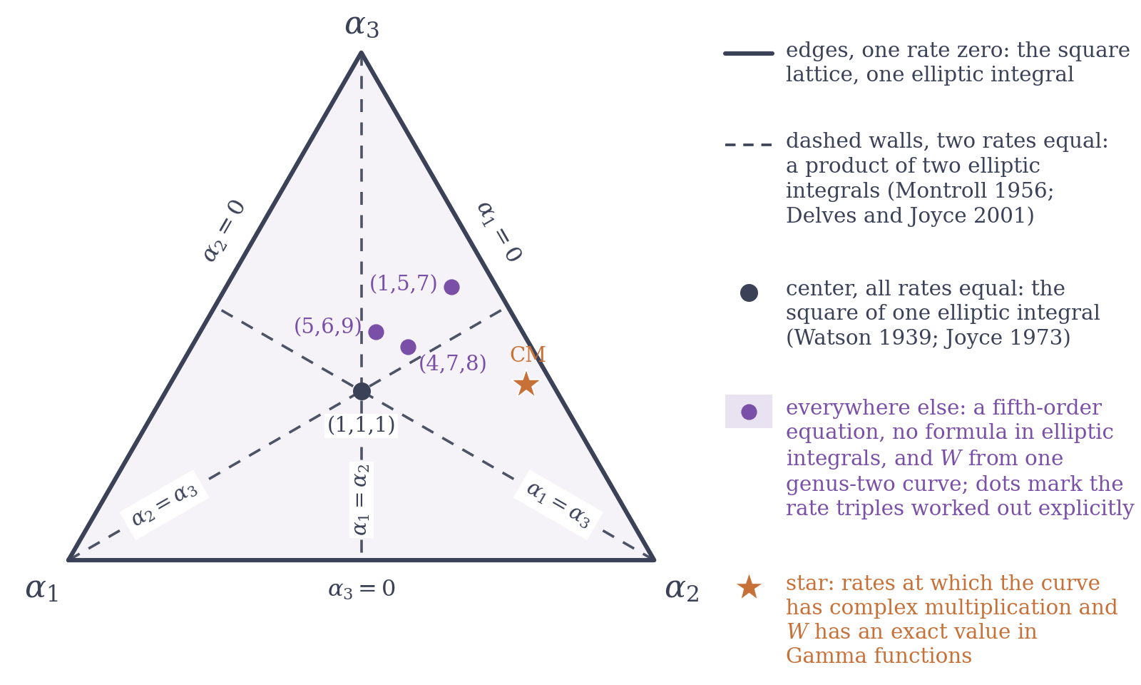
The map of hopping rates. Only the ratio $\alpha_1:\alpha_2:\alpha_3$ of the three rates matters for the shape of the answer, so every anisotropic lattice is a point of this triangle, with $w$ running along a ray over each point. On the edges one rate is zero and the walk lives on a square lattice. On the dashed walls two rates are equal, and $w\,W$ is an algebraic function times a product of two complete elliptic integrals; at the center all three are equal and it is the square of one. The first main result concerns every other point, away from a further countable set of algebraic curves: there $W$ satisfies a fifth-order equation in $w$ whose symmetry group has connected part $\mathrm{SO}(5)$, and no formula in elliptic integrals exists. The violet dots are rate triples at which the formula has been worked out explicitly; the orange star marks the rates at which the genus-two curve has complex multiplication and $W$ has an exact value in Gamma functions.
The proof that no formula in elliptic integrals exists for generic rates turns on the order of the differential equation in $w$. $K(k)$ is a perioda number obtained by integrating an algebraic differential form over a closed cycle of an algebraic curve or surface; Feynman integrals in particle physics are periods in the same sense of a torus, the curve $y^2=(1-t^2)(1-k^2t^2)$: the integral of $\mathrm dt/y$ around one of its two independent loops. Two loops give two periods, both satisfying one second-order equation; a square then satisfies an equation of order three, a product order four. In each solved case the order counts the independent cycles carrying a nonzero period. One can search for a product formula and find one, but a failed search proves nothing; the symmetry group of the differential equation, which records how its solutions mix among themselves when continued around the singular points, can prove that none exists.
A surface with five periods
For the three-angle Watson integrand the analogue of the torus is a surface. With the angles complex, the denominator vanishes on a surface of two complex dimensions, and $W$ is a period of it: the integral of the residue of the integrand, a two-form, over a closed two-cycle. In the variables $z_j=e^{ik_j}$ the surface is $a\,z_2z_3(z_1^2+1)+b\,z_1z_3(z_2^2+1)+c\,z_1z_2(z_3^2+1)=2z_1z_2z_3$, with $a,b,c$ the rates divided by $w$. It has eight ordinary double pointsthe simplest singular point of a surface, shaped locally like the tip of a cone; smoothing replaces the tip by a small sphere at the corners where every $z_i$ is $0$ or $\infty$, and smoothing them gives a K3 surface, a simply connected complex surface carrying a nowhere-vanishing holomorphic two-form: the two-dimensional analogue of an elliptic curve. Call it the Watson K3; Koike had studied the family in 2011, and his description of its cycles is used throughout.
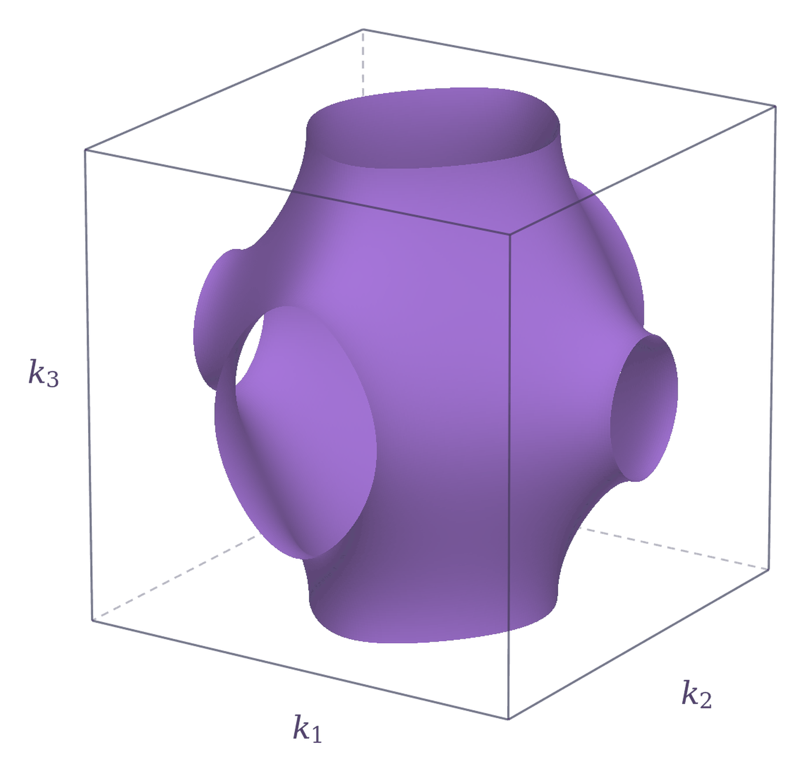
The surface on which the Watson integrand becomes infinite, $\alpha_1\cos k_1+\alpha_2\cos k_2+\alpha_3\cos k_3=w$, drawn as its real points in one cube of crystal momenta, $-\pi\le k_i\le\pi$ (a Brillouin zone), for rates $(\alpha_1,\alpha_2,\alpha_3)=(1,0.8,0.6)$ and $w=0.15$. That value of $w$ lies inside the band, so real momenta solve the equation and the picture is a constant-energy surface of the tight-binding band; the tubes continue periodically into the neighboring cubes, widest along the axis with the smallest rate. For the walk $w$ sits above the band, no real momentum solves the equation, and the momenta must be taken complex: the complex surface, with its eight corner singularities smoothed, is the Watson K3 surface, and $W$ is one of its periods. (Plotted from the equation for this page.)
A K3 surface has twenty-two independent two-cycles, but the two-form integrates to zero over any cycle traced out by an algebraic curve on the surface. For every choice of rates, the twelve coordinate lines on the surface and the eight curves created by smoothing the double points generate seventeen independent algebraic classes; for very general rates, meaning outside a countable collection of algebraic exceptions, there are no others. So $22-17=5$ periods survive, one of them $w\,W$, and at fixed rates they span the solutions of a fifth-order linear differential equation in $w$, the Picard–Fuchs equation, which can be written out in full:
$$\mathcal L_5\,\big[\,w\,W\,\big]=0,\qquad \mathcal L_5=\sum_{k=0}^{6}x^{k}\,\mathsf P_k(\vartheta),\qquad \mathsf P_0=\vartheta^{3}(\vartheta-1)(\vartheta-2),\qquad \vartheta=x\frac{\mathrm d}{\mathrm dx},\qquad x=\frac{1}{w^{2}}\,.$$In words: $\vartheta$ is the derivative that counts powers of $x=1/w^2$, and each $\mathsf P_k$ is a polynomial of degree at most five in $\vartheta$ with coefficients polynomial in the symmetric functions of the squared rates. Because the series coefficients of $w\,W$ are exact, $\mathcal L_5[wW]=0$ can be checked term by term. The genuine singular points are the eight thresholds $w=\pm\alpha_1\pm\alpha_2\pm\alpha_3$, the outermost two being the band edges, where the surface acquires an extra double point.
The first main result is that for a very general direction of rates $(\alpha_1^2:\alpha_2^2:\alpha_3^2)$ the minimal equation for $w\,W$ is $\mathcal L_5$, irreduciblenot factorable into differential operators of lower order: no smaller equation with algebraic coefficients is satisfied by any of its solutions, with the full group $\mathrm{SO}(5)$ as the connected part of its symmetry group. The proof is Hodge-theoreticit argues from the position of the holomorphic two-form relative to the surface’s integer cycles and how it moves with the rates, not from formulas: results of Zarhin and André leave no room for hidden symmetries of the five transcendental cyclesthe cycles not coming from algebraic curves on the surface, the only ones with nonzero periods; their count gives the order of the differential equation or of their monodromythe way the solutions of a linear differential equation are reshuffled among themselves when the variable is carried around a loop enclosing a singular point; for a family of algebraic surfaces it is given by integer matrices acting on the cycles along the ray. The five solutions then mix under analytic continuation as freely as five functions bound by one quadratic relation can, and no expression in complete elliptic integrals of algebraic moduli, products and symmetric powers included, can do that. Such an expression would confine the group to one built from copies of $\mathrm{SL}(2)$, the group belonging to a single elliptic integral. The theorem does not cover the walls, nor a further countable set of rate directions that the proof leaves unspecified.
The count of transcendental cycles also accounts for the classical formulas. On a wall $\alpha_i=\alpha_j$ one more cycle becomes algebraic, only four periods still vary with $w$, and up to a finite cover the group is $\mathrm{SL}(2)\times\mathrm{SL}(2)$, whose periods are products of elliptic periods: the Delves–Joyce formula with its fourth-order equation. On the diagonal three periods remain and the system is the symmetric square of one elliptic system: Joyce’s isotropic square, of order three.
A curve of genus two
The group $\mathrm{SO}(5)$ forbids elliptic curves but permits one other construction, through the coincidence of Lie algebras $\mathfrak{so}(5)\simeq\mathfrak{sp}(4)$. Five functions bound by one quadratic relation can be written as the $2\times2$ minors of a $2\times4$ matrix. A curve of genus two, $y^2=f(t)$ with $f$ of degree six rather than three or four, has exactly such a period matrix: two holomorphic one-forms integrated around four independent loops. Which genus-two curve plays this role is determined by the rates.
Doing the $k_3$ integral first shows that $W$ is also a period of a double cover of the plane branched along six lines. For that family Matsumoto and Terasoma expressed the squared theta constants, special values of Riemann’s theta functions that serve as coordinates on the space of period matrices, through the coefficients of the lines. From the ratios of these theta constants and Thomae’s classical formula one obtains the Igusa–Clebsch invariantsfour numbers built from the coefficients of the sextic that determine a genus-two curve up to isomorphism, as the j-invariant determines an elliptic curve that determine the curve. They come out as explicit polynomials in the symmetric functions of $a^2,b^2,c^2$ and in one square root, that of the product $q$ of the eight normalized thresholds $1\pm a\pm b\pm c$. The two signs of $\sqrt q$ give two curves, $C_-$ and $C_+$, related by a Richelot isogeny, the genus-two version of Landen’s transformation of elliptic integrals. An explicit construction then gives a real model of either curve with six real branch points, by three successive square roots in the squared rates, throughout the chamber $\alpha_1+\alpha_2+\alpha_3\lt w$. On such a model,
$$W(\alpha_1,\alpha_2,\alpha_3;w)\;=\;\frac{|\Delta|}{4\pi^{2}\,w}\,\Big[\,p_0(J_1)\,p_1(J_2)-p_1(J_1)\,p_0(J_2)\Big],$$ $$p_g(J)=2\int_J\frac{t^{g}\,\mathrm dt}{\sqrt{|f(t)|}}\,,\qquad f=G_1G_2G_3\,,\qquad \alpha_1+\alpha_2+\alpha_3\lt w\,.$$Here $f$ is a real sextic with six real roots, factored into three real quadratics $G_1,G_2,G_3$, one belonging to each rate by an explicit algebraic test, and $\Delta$ is the $3\times3$ determinant of their coefficients. $J_1$ and $J_2$, with $J_1$ to the left, are two of the gaps between consecutive roots, each bounded by roots of two different factors, and the $p_g(J)$ are complete hyperelliptic integrals over them: ordinary one-dimensional integrals, the genus-two counterparts of $K(k)$. The bracket is a $2\times2$ minor of the curve’s period matrix, and $|\Delta|$ times it does not depend on the model. As written the formula holds on $C_-$; on $C_+$ the coefficient is halved and a different pair of gaps is used. It is a closed formula in the rates and $w$: square roots give the curve, and four one-dimensional integrals give the Green’s function at every energy above the band.
At rates $(1,5,7)$ and $w=17$ the product of the eight thresholds $w\pm\alpha_1\pm\alpha_2\pm\alpha_3$ is the perfect square $(8!)^2$, so the invariants of both curves are rational numbers, and here models with rational coefficients exist; one for $C_-$ is $v^2=(2r-1)(r^2+5r+1)(14r^2-2r-1)$ with $\Delta=102$, and the formula reads $2\pi^2\,W(1,5,7;17)=3\,[\,p_0(J_1)p_1(J_2)-p_1(J_1)p_0(J_2)\,]$. The right side reproduces the value $W(1,5,7;17)=0.0699642768\ldots$ obtained independently from the Bessel-function form of the integral, to all twenty-five digits of that computation, and in a separate comparison the two sides agree to 35–40 digits for this and three further rate tuples. These digit counts are numerical checks only, not rigorous error bounds, and the proof does not use them.
Fixing the constant
The genus-two curve fixes $W$ only up to normalization: which cycles give the original integral, and what constant stands in front, must still be determined, and the return probability depends on both. The two are settled together, with one exact evaluation and a continuity argument. The evaluation is at a curve with complex multiplicationa rare extra symmetry of an elliptic curve or of the Jacobian of a genus-two curve: extra endomorphisms by an imaginary quadratic field or, for genus two, a quartic CM field. It is the mechanism behind the classical evaluations of periods in values of the gamma function at rational arguments (the Chowla–Selberg formula and its descendants), $v^2=(u+2)(u^4-4u^2+2)$, taken from van Wamelen’s list of such curves over the rationals. Its Jacobian (the complex torus built from the curve’s periods) has multiplication by the quartic field generated by a root of $\eta^4+4\eta^2+2=0$, of conductor 16. Its six branch points, grouped into adjacent pairs, match an explicit rate triple built from $\sqrt2$, $\sqrt5$ and $t_{16}=\sqrt{2-\sqrt2}$: three distinct nonzero rates off every wall, the star in the triangle of rates above. The curve’s periods reduce to Euler beta integrals, which give $W$ at these rates in Gamma functions: $\sqrt5\,W(\alpha_{1,*},\alpha_{2,*},\alpha_{3,*};w_*)=\frac{\sqrt2\,(1+t_{16})}{64\pi^3}\,\Gamma(\tfrac1{16})\Gamma(\tfrac3{16})\Gamma(\tfrac5{16})\Gamma(\tfrac7{16})$, numerically $W_*=0.248456466441\ldots$.
The delicate part is the absolute normalization. The walk and the CM curve each give a point in the period domain of the six-line family with its squared theta constants known exactly, one by the Matsumoto–Terasoma formula and the other by Thomae’s classical one. The two points can differ only by a discrete symmetry, which rescales the theta squares by a positive factor $\lambda$. One proves that any such factor is either exactly $1$ or at least $2$; crude rational bounds give $\lambda\lt161/100$; hence $\lambda=1$. A seven-step continuation argument, in which the six branch points stay real and distinct throughout the chamber, then extends the identity to all rates and from $C_+$ to $C_-$. The outcome is the “constant law”: the displayed formula with its coefficients fixed for all positive rates with $\alpha_1+\alpha_2+\alpha_3\lt w$. It holds on the walls too, alongside the Delves–Joyce product, though the two have not been reduced to one another directly.
The constant law extends by continuity to the band edge $w=w^\star$, where $q=0$ and the two curves merge into one smooth genus-two curve. For rates in the ratio $1:5:7$ the merged curve has an explicit model with coefficients involving $\sqrt{39}$. The formula gives $W(1,5,7;13)=0.1372148875\ldots$, and both forms of the law, on $C_-$ and on $C_+$, agree with the Bessel-function form of the integral to thirty digits. The return probability is then $1-1/[13\,W(1,5,7;13)]=0.4393970047\ldots$: a walker hopping at rates $1:5:7$ comes home with probability $0.4393\ldots$, against $0.3405\ldots$ at equal rates.
Kummer surfaces and open questions
The Watson K3 surface itself is also related to the two curves, although the formula for $W$ does not need this. Every genus-two curve yields a K3 surface, its Kummer surface: form the complex torus generated by the curve’s periods, identify each point with its negative, and smooth the sixteen singular points. For very general rates the Watson K3 is not a Kummer surface. Instead the Kummer surface of either curve covers it four-to-one, and it in turn covers two-to-one the Kummer surfaces of three complex tori that sit halfway along the Richelot isogeny; these three are its quotients by the symmetries reversing two of the three lattice directions. This tower of coverings explains why the rates determine two curves rather than one, and why rates, lattice directions and quadratic factors $G_i$ correspond one to one.
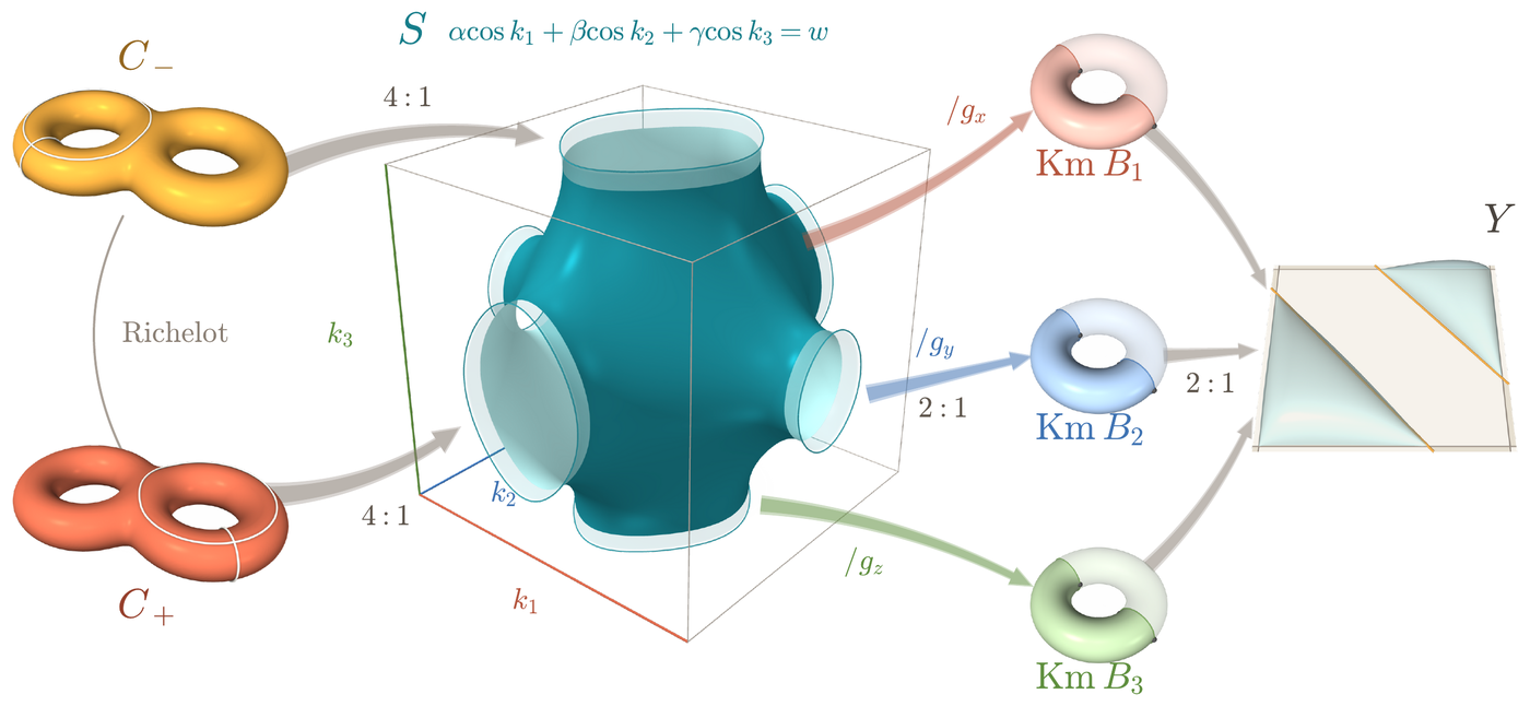
The tower of surfaces attached to one lattice, here with rates $(\alpha_1,\alpha_2,\alpha_3)=(1,0.8,0.6)$, written $\alpha,\beta,\gamma$ in the figure. Center: the singular surface $S$ of the integrand in one cube of momenta, the surface of the previous figure, standing for the Watson K3. Left: the two genus-two curves $C_-$ and $C_+$ fixed by the rates, joined by the Richelot isogeny; each stands for the Kummer surface of its Jacobian, and each of those covers $S$ four-to-one. Right: dividing $S$ by the symmetry that reverses two of the three lattice directions gives a Kummer surface, $\mathrm{Km}\,B_1$, $\mathrm{Km}\,B_2$ or $\mathrm{Km}\,B_3$ according to the direction left alone, by a two-to-one map. Each of these covers two-to-one the surface $Y$ at the far right: the double cover of the plane branched along six lines that appears when the $k_3$ integral is done first, drawn with its branch lines. An arrow marked $4{:}1$ or $2{:}1$ means that many points above each point below. The curves and Kummer surfaces are drawn schematically as tori; the degrees are exact.
The order-five result with its $\mathrm{SO}(5)$ group, the invariants of the two curves, the Gamma value at the conductor-16 point with its absolute normalization, and the constant law throughout the chamber and at the band edge are all proved. One further statement is a conjecture: an absolute theta identity, $(1-a^2-b^2-c^2)\,(wW)^2=\Theta_{\rm K}(\tau)$, equating the left side with Koike’s weight-two theta function at the period point. It holds to more than 160 digits at seven rate tuples, and the constant law does not depend on it. Several questions remain open: the values of $W$ at points with complex multiplication by $\mathbb Q(\zeta_5)$, which should come out in $\Gamma(j/5)$; whether the grouping of the six roots into three quadratics, one for each rate, is always unique; and the expansion of the closed form at the band edge. The authors used AI tools interactively in the work, noting that the tools’ plausible statements require the same scrutiny as any other proposed proof.
The paper
- The anisotropic Watson integral — Noam Elkies, Thomas W. Grimm and Matthew D. Schwartz; in preparation.
Supplementary material
The two files below give the closed form as a short program, in Mathematica and in Python (both files derive from SageMath's implementation of Mestre's construction and are released under the GPL, version 2 or later); every value is recomputed live at the precision requested and no digit strings enter the computation.
- WatsonW.wl — The formula in executable form, 84 lines of Mathematica:
WatsonW[w, α1, α2, α3]runs the seven steps (symmetric functions of the squared rates, the threshold quartic and its marked branch, the four Igusa–Clebsch invariants, a real sextic model by Mestre’s construction, the marked partition and its determinant $\Delta$, the two period integrals and the minor $M$) and returns $W=|\Delta M|/(4\pi^{2}w)$. Load withGet["WatsonW.wl"];WatsonW[17, 1, 5, 7]returns 0.0699642768…Show the Mathematica code
(* SPDX-License-Identifier: GPL-2.0-or-later Derived from SageMath (https://www.sagemath.org), sage/schemes/hyperelliptic_curves/mestre.py (Florian Bouyer, Marco Streng; Copyright (C) 2011-2013, and 2025 Sabrina Kunzweiler, Gareth Ma, Giacomo Pope) and invariants.py (Nick Alexander; Copyright (C) 2008), licensed under the GNU General Public License v2.0 or later. This Wolfram Language transliteration of Mestre's conic-and-cubic construction keeps SageMath's conventions and normalizations. It is Copyright (c) 2026 Anthropic, PBC; created by Matthew D. Schwartz, code written by Claude (Anthropic) under his supervision, and is distributed under the same GNU General Public License v2.0 or later. The license text is LICENSE-GPL-2.0 beside this file; the rest of the bundle is MIT (see NOTICE). *) (* WatsonW[w, a, b, c]: the anisotropic simple-cubic Watson integral in closed form, W = |Delta M|/(4 Pi^2 w), for rates a, b, c = alpha_1, alpha_2, alpha_3 and spectral variable w. WatsonW[17, 1, 5, 7] = 0.069964276874484951... *) MestreSextic[i2_, i4_, i6_, i10_, t_, sgn_: 1] := Module[{x, y, z, L, es, ord, P, V, U, s, c, f}, x = 8 (1 + 20 i4/i2^2)/225; y = 16 (1 + 80 i4/i2^2 - 600 i6/i2^3)/3375; z = -64 (-10800000 i10/i2^5 - 9 - 700 i4/i2^2 + 3600 i6/i2^3 + 12400 i4^2/i2^4 - 48000 i4 i6/i2^5)/253125; L = N[{{x + 6 y, 6 x^2 + 2 y, 2 z}, {6 x^2 + 2 y, 2 z, 9 x^3 + 4 x y + 6 y^2}, {2 z, 9 x^3 + 4 x y + 6 y^2, 6 x^2 y + 2 y^2 + 3 x z}}, 40]; es = Eigensystem[L]; ord = Ordering[es[[1]]]; P = es[[2, ord[[3]]]]/Sqrt[es[[1, ord[[3]]]]] + sgn es[[2, ord[[1]]]]/Sqrt[-es[[1, ord[[1]]]]]; V = {0, 1, s}; U = (V.L.V) P - 2 (P.L.V) V; c = {{1, 1, 1} -> 12 x y - 2 y/3 - 4 z, {1, 1, 2} -> -18 x^3 - 12 x y - 36 y^2 - 2 z, {1, 1, 3} -> -9 x^3 - 36 x^2 y - 4 x y - 6 x z - 18 y^2, {1, 2, 2} -> -9 x^3 - 36 x^2 y - 4 x y - 6 x z - 18 y^2, {1, 2, 3} -> -54 x^4 - 36 x^2 y - 36 x y^2 - 6 x z - 4 y^2 - 24 y z, {1, 3, 3} -> -27 x^4/2 - 72 x^3 y - 6 x^2 y - 9 x^2 z - 39 x y^2 - 36 y^3 - 2 y z, {2, 2, 2} -> -27 x^4 - 18 x^2 y - 6 x y^2 - 8 y^2/3 + 2 y z, {2, 2, 3} -> 9 x^3 y - 27 x^2 z + 6 x y^2 + 18 y^3 - 8 y z, {2, 3, 3} -> -81 x^5/2 - 27 x^3 y - 9 x^2 y^2 - 4 x y^2 + 3 x y z - 6 z^2, {3, 3, 3} -> 27 x^4 y/2 - 27 x^3 z/2 + 9 x^2 y^2 + 3 x y^3 - 6 x y z + 4 y^3/3 - 10 y^2 z}; f = Total[(#[[2]] U[[#[[1, 1]]]] U[[#[[1, 2]]]] U[[#[[1, 3]]]]) & /@ c]; Expand[f] /. s -> t]; WatsonW[w_, a_, b_, c_] := Module[ {e1, e2, e3, x, q4, rr, i2, i4, i6, i10, t, f, r, sgn, lc, prs, qd, score, best, g1, g2, g3, dd, cutQ, seg, p, mm}, {e1, e2, e3} = {a^2 + b^2 + c^2, a^2 b^2 + a^2 c^2 + b^2 c^2, a^2 b^2 c^2}; x = 1/w^2; q4 = e1^4 x^4 - 4 e1^3 x^3 - 8 e1^2 e2 x^4 + 6 e1^2 x^2 + 16 e1 e2 x^3 + 16 e2^2 x^4 - 8 e2 x^2 - 64 e3 x^3 - 4 e1 x + 1; rr = -Sqrt[q4]; i2 = 48 e1^2 x^2 - 32 e1 x - 192 e2 x^2 + 80 - 48 rr; i4 = 544 e1^2 x^2 - 1088 e1 x - 1152 e2 x^2 + 544 - 480 rr; i6 = 16384 e1^4 x^4 - 48384 e1^3 x^3 - 114688 e1^2 e2 x^4 + 64256 e1^2 x^2 + 177152 e1 e2 x^3 - 48896 e1 x + 196608 e2^2 x^4 - 99328 e2 x^2 - 417792 e3 x^3 + 16640 + (-16384 e1^2 x^2 + 17152 e1 x + 49152 e2 x^2 - 16128) rr; i10 = 32768 e3 x^3 (e1^2 x^2 - 2 e1 x - 4 e2 x^2 + 1 + rr); sgn = 1; f = MestreSextic[i2, i4, i6, i10, t, sgn]; r = t /. NSolve[f == 0, t, WorkingPrecision -> 40]; If[Max[Abs[Im[r]]] > 10^-10, sgn = -1; f = MestreSextic[i2, i4, i6, i10, t, sgn]; r = t /. NSolve[f == 0, t, WorkingPrecision -> 40]]; r = Sort[Re[r]]; lc = Coefficient[f, t, Exponent[f, t]]; prs = {{1,2,3,4,5,6}, {1,3,2,4,5,6}, {1,4,2,3,5,6}, {1,2,3,5,4,6}, {1,2,3,6,4,5}, {1,3,2,5,4,6}, {1,3,2,6,4,5}, {1,4,2,5,3,6}, {1,4,2,6,3,5}, {1,5,2,3,4,6}, {1,5,2,4,3,6}, {1,5,2,6,3,4}, {1,6,2,3,4,5}, {1,6,2,4,3,5}, {1,6,2,5,3,4}}; qd[{i_, j_}] := (t - r[[i]]) (t - r[[j]]); score[pr_] := Module[{u1, u2, u3, v, tgt}, {u1, u2, u3} = qd /@ {pr[[{1, 2}]], pr[[{3, 4}]], pr[[{5, 6}]]}; v = Sort[Abs[{Discriminant[u1, t] Resultant[u2, u3, t], Discriminant[u2, t] Resultant[u3, u1, t], Discriminant[u3, t] Resultant[u1, u2, t]}]]; tgt = Sort[N[x {a^2, b^2, c^2}, 40]]; Max[v/tgt]/Min[v/tgt]]; best = First[MinimalBy[prs, score]]; {g1, g2, g3} = qd /@ {best[[{1, 2}]], best[[{3, 4}]], best[[{5, 6}]]}; dd = lc Det[Table[Coefficient[{g1, g2, g3}[[k]], t, m], {k, 3}, {m, {2, 1, 0}}]]; cutQ = best[[2]] == best[[1]] + 1 && best[[4]] == best[[3]] + 1; seg = If[cutQ, {{r[[2]], r[[3]]}, {r[[4]], r[[5]]}}, {{r[[1]], r[[2]]}, {r[[3]], r[[4]]}}]; p[gg_, {u_, v_}] := 2 NIntegrate[t^gg/Sqrt[Abs[f]], {t, u, v}, WorkingPrecision -> 30]; mm = p[0, seg[[1]]] p[1, seg[[2]]] - p[1, seg[[1]]] p[0, seg[[2]]]; Abs[dd mm]/(4 Pi^2 w)]; - WatsonW.py — The same program in Python (mpmath only, 118 lines), the same steps in the same order:
python3 WatsonW.pyprintsWatsonW(17, 1, 5, 7)= 0.0699642768…Show the Python code
# SPDX-License-Identifier: GPL-2.0-or-later
#
# Derived from SageMath (https://www.sagemath.org),
# sage/schemes/hyperelliptic_curves/mestre.py (Florian Bouyer, Marco Streng; Copyright (C)
# 2011-2013, and 2025 Sabrina Kunzweiler, Gareth Ma, Giacomo Pope) and invariants.py (Nick
# Alexander; Copyright (C) 2008), licensed under the GNU General Public License v2.0 or
# later. This Python transliteration of Mestre's conic-and-cubic construction keeps
# SageMath's conventions and normalizations. It is Copyright (c) 2026 Anthropic, PBC;
# created by Matthew D. Schwartz, code written by Claude (Anthropic) under his supervision,
# and is distributed under the same GNU General Public License v2.0 or later. The license
# text is LICENSE-GPL-2.0 beside this file; the rest of the bundle is MIT (see NOTICE).

# WatsonW(w, a, b, c): the anisotropic simple-cubic Watson integral in closed form, W = |Delta M|/(4 pi^2 w),
# for rates a, b, c = alpha_1, alpha_2, alpha_3 and spectral variable w; mpmath only.
# python3 WatsonW.py prints WatsonW(17, 1, 5, 7) = 0.069964276874484951...
from mpmath import mp, mpf, sqrt, pi, matrix, eigsy, polyroots, fprod, det, quad, sin, fabs, im, re

# Polynomials in one variable are coefficient lists, highest power first (the convention of polyroots).
def polmul(p, q):
    r = [0]*(len(p) + len(q) - 1)
    for i, u in enumerate(p):
        for j, v in enumerate(q): r[i + j] += u*v
    return r
def poladd(p, q):
    n = max(len(p), len(q)); p, q = [0]*(n - len(p)) + p, [0]*(n - len(q)) + q
    return [u + v for u, v in zip(p, q)]
def polscale(k, p): return [k*u for u in p]

# MestreSextic(i2, i4, i6, i10, sgn) returns the coefficients of a sextic f(t) whose genus-two curve
# y^2 = f(t) has Igusa-Clebsch invariants (i2 : i4 : i6 : i10): Mestre's conic-and-cubic construction,
# with sgn selecting between the two real points used on the conic. WatsonW tries sgn = 1 and falls
# back to sgn = -1 so that all six roots of f are real.
def MestreSextic(i2, i4, i6, i10, sgn=1):
    x = 8*(1 + 20*i4/i2**2)/225
    y = 16*(1 + 80*i4/i2**2 - 600*i6/i2**3)/3375
    z = -64*(-10800000*i10/i2**5 - 9 - 700*i4/i2**2 + 3600*i6/i2**3 + 12400*i4**2/i2**4 - 48000*i4*i6/i2**5)/253125
    L = matrix([[x + 6*y, 6*x**2 + 2*y, 2*z],
                [6*x**2 + 2*y, 2*z, 9*x**3 + 4*x*y + 6*y**2],
                [2*z, 9*x**3 + 4*x*y + 6*y**2, 6*x**2*y + 2*y**2 + 3*x*z]])
    E, Q = eigsy(L)                      # eigenvalues ascending, orthonormal eigenvectors in the columns
    P = [Q[k, 2]/sqrt(E[2]) + sgn*Q[k, 0]/sqrt(-E[0]) for k in range(3)]
    V = [[0], [1], [1, 0]]               # V = (0, 1, s), each entry a polynomial in s
    VLV = [L[2, 2], 2*L[1, 2], L[1, 1]]  # V.L.V
    LP = [sum(L[i, k]*P[k] for k in range(3)) for i in range(3)]
    PLV = [LP[2], LP[1]]                 # P.L.V
    U = [poladd(polscale(P[i], VLV), polscale(-2, polmul(PLV, V[i]))) for i in range(3)]
    c = {(1, 1, 1): 12*x*y - 2*y/3 - 4*z,
         (1, 1, 2): -18*x**3 - 12*x*y - 36*y**2 - 2*z,
         (1, 1, 3): -9*x**3 - 36*x**2*y - 4*x*y - 6*x*z - 18*y**2,
         (1, 2, 2): -9*x**3 - 36*x**2*y - 4*x*y - 6*x*z - 18*y**2,
         (1, 2, 3): -54*x**4 - 36*x**2*y - 36*x*y**2 - 6*x*z - 4*y**2 - 24*y*z,
         (1, 3, 3): -27*x**4/2 - 72*x**3*y - 6*x**2*y - 9*x**2*z - 39*x*y**2 - 36*y**3 - 2*y*z,
         (2, 2, 2): -27*x**4 - 18*x**2*y - 6*x*y**2 - 8*y**2/3 + 2*y*z,
         (2, 2, 3): 9*x**3*y - 27*x**2*z + 6*x*y**2 + 18*y**3 - 8*y*z,
         (2, 3, 3): -81*x**5/2 - 27*x**3*y - 9*x**2*y**2 - 4*x*y**2 + 3*x*y*z - 6*z**2,
         (3, 3, 3): 27*x**4*y/2 - 27*x**3*z/2 + 9*x**2*y**2 + 3*x*y**3 - 6*x*y*z + 4*y**3/3 - 10*y**2*z}
    f = [0]
    for (i, j, k), cijk in c.items():
        f = poladd(f, polscale(cijk, polmul(polmul(U[i - 1], U[j - 1]), U[k - 1])))
    return f

# WatsonW(w, alpha_1, alpha_2, alpha_3), the seven steps of the closed form. The sextic is built at dps + 30 digits
# (Mestre's construction loses up to about twenty-five digits at these tuples), the period integrals at dps.
def WatsonW(w, a, b, c, dps=30):
    mp.dps = dps + 30
    w, a, b, c = mpf(w), mpf(a), mpf(b), mpf(c)
    # (i) elementary symmetric functions e1, e2, e3 of the squared rates and x = 1/w^2
    e1, e2, e3 = a**2 + b**2 + c**2, a**2*b**2 + a**2*c**2 + b**2*c**2, a**2*b**2*c**2
    x = 1/w**2
    # (ii) the threshold quartic Q4 and the marked branch R = -sqrt(Q4)
    q4 = (e1**4*x**4 - 4*e1**3*x**3 - 8*e1**2*e2*x**4 + 6*e1**2*x**2 + 16*e1*e2*x**3
          + 16*e2**2*x**4 - 8*e2*x**2 - 64*e3*x**3 - 4*e1*x + 1)
    rr = -sqrt(q4)
    # (iii) the four Igusa-Clebsch invariants in closed form, polynomials in e1, e2, e3, x, R
    i2 = 48*e1**2*x**2 - 32*e1*x - 192*e2*x**2 + 80 - 48*rr
    i4 = 544*e1**2*x**2 - 1088*e1*x - 1152*e2*x**2 + 544 - 480*rr
    i6 = (16384*e1**4*x**4 - 48384*e1**3*x**3 - 114688*e1**2*e2*x**4 + 64256*e1**2*x**2
          + 177152*e1*e2*x**3 - 48896*e1*x + 196608*e2**2*x**4 - 99328*e2*x**2
          - 417792*e3*x**3 + 16640 + (-16384*e1**2*x**2 + 17152*e1*x + 49152*e2*x**2 - 16128)*rr)
    i10 = 32768*e3*x**3*(e1**2*x**2 - 2*e1*x - 4*e2*x**2 + 1 + rr)
    # (iv) a real sextic model from MestreSextic, sgn = 1 then -1 so that all six roots are real
    sgn = 1; f = MestreSextic(i2, i4, i6, i10, sgn)
    r = polyroots(f, maxsteps=200, extraprec=200)
    if max(fabs(im(z)) for z in r) > mpf(10)**-10:
        sgn = -1; f = MestreSextic(i2, i4, i6, i10, sgn)
        r = polyroots(f, maxsteps=200, extraprec=200)
    r = sorted(re(z) for z in r)
    lc = f[0]
    # (v) the marked partition into three real quadratics, by the disc-resultant normalization test
    #     against x {a^2, b^2, c^2}, and its determinant Delta (quadratics monic, from pairs of roots)
    prs = [(1,2,3,4,5,6), (1,3,2,4,5,6), (1,4,2,3,5,6), (1,2,3,5,4,6), (1,2,3,6,4,5),
           (1,3,2,5,4,6), (1,3,2,6,4,5), (1,4,2,5,3,6), (1,4,2,6,3,5), (1,5,2,3,4,6),
           (1,5,2,4,3,6), (1,5,2,6,3,4), (1,6,2,3,4,5), (1,6,2,4,3,5), (1,6,2,5,3,4)]
    disc = lambda i, j: (r[i-1] - r[j-1])**2
    res = lambda i, j, k, l: (r[i-1] - r[k-1])*(r[i-1] - r[l-1])*(r[j-1] - r[k-1])*(r[j-1] - r[l-1])
    def score(pr):
        i, j, k, l, m, n = pr
        v = sorted(fabs(u) for u in [disc(i, j)*res(k, l, m, n), disc(k, l)*res(m, n, i, j), disc(m, n)*res(i, j, k, l)])
        tgt = sorted([x*a**2, x*b**2, x*c**2])
        q = [v[s]/tgt[s] for s in range(3)]
        return max(q)/min(q)
    best = min(prs, key=score)
    g = [[1, -(r[i-1] + r[j-1]), r[i-1]*r[j-1]] for i, j in (best[0:2], best[2:4], best[4:6])]
    dd = lc*det(matrix(g))
    # (vi) the two integration segments by the cyclic-adjacency rule and the period minor M
    cutQ = best[1] == best[0] + 1 and best[3] == best[2] + 1
    seg = [(r[1], r[2]), (r[3], r[4])] if cutQ else [(r[0], r[1]), (r[2], r[3])]
    mp.dps = dps
    def p(gg, u, v):   # p_g(J) = 2 int_J t^g dt/sqrt|f|, with t = u + (v - u) sin^2(theta): the square-root
        others = [ri for ri in r if ri != u and ri != v]   # endpoint factors cancel against dt and the
        tt = lambda th: u + (v - u)*sin(th)**2            # quadrature converges to the working precision
        return 4*quad(lambda th: tt(th)**gg/sqrt(fabs(lc*fprod(tt(th) - ri for ri in others))), [0, pi/2])
    mm = p(0, *seg[0])*p(1, *seg[1]) - p(1, *seg[0])*p(0, *seg[1])
    # (vii) W_S = |Delta M| / (4 pi^2 w)
    return fabs(dd*mm)/(4*pi**2*w)

if __name__ == "__main__":
    print("WatsonW(17, 1, 5, 7) =", mp.nstr(WatsonW(17, 1, 5, 7), 20))
References
| G. Pólya, Über eine Aufgabe der Wahrscheinlichkeitsrechnung betreffend die Irrfahrt im Straßennetz, Math. Ann. 84 (1921) 149 | return is certain on the line and the square grid, not on the cubic lattice |
| G. N. Watson, Three triple integrals, Q. J. Math. (Oxford) 10 (1939) 266 | the cubic-lattice integrals in complete elliptic integrals; the subject’s namesake |
| E. W. Montroll, Theory of the vibration of simple cubic lattices with nearest neighbor interactions, in Proc. Third Berkeley Symp. Math. Stat. Prob., vol. 3, Univ. California Press (1956) 209 | the tetragonal band-edge value |
| G. S. Joyce, On the simple cubic lattice Green function, Phil. Trans. R. Soc. Lond. A 273 (1973) 583 | the isotropic Green’s function at every $w$ as the square of one elliptic integral |
| M. L. Glasser and I. J. Zucker, Extended Watson integrals for the cubic lattices, Proc. Natl. Acad. Sci. USA 74 (1977) 1800 | Watson’s value in gamma functions |
| R. T. Delves and G. S. Joyce, On the Green function for the anisotropic simple cubic lattice, Ann. Phys. 291 (2001) 71 | the tetragonal line: a product $K(k_+)K(k_-)$ of two elliptic integrals |
| A. J. Guttmann, Lattice Green functions in all dimensions, J. Phys. A 43 (2010) 305205 | survey of lattice Green’s functions and their differential equations |
| I. J. Zucker, 70+ years of the Watson integrals, J. Stat. Phys. 145 (2011) 591 | the survey that named the orthorhombic case “the final problem” |
| K. Koike, Hessian K3 surfaces of non-Sylvester type, J. Algebra 330 (2011) 388 | the family of K3 surfaces to which the Watson K3 belongs, with its cycles and its theta function |
| K. Matsumoto and T. Terasoma, Thomae type formula for K3 surfaces given by double covers of the projective plane branching along six lines, J. reine angew. Math. 669 (2012) 121 | the exact theta constants of the six-line family used to fix the normalization |
| P. van Wamelen, Examples of genus two CM curves defined over the rationals, Math. Comp. 68 (1999) 307 | the list of curves with complex multiplication from which the conductor-16 curve is taken |
| J.-F. Mestre, Construction de courbes de genre 2 à partir de leurs modules, in Effective Methods in Algebraic Geometry, Progr. Math. 94 (1991) 313 | rebuilding a genus-two curve from its invariants; used to write rational models of the curve at sample rates |
| J.-i. Igusa, Arithmetic variety of moduli for genus two, Ann. Math. 72 (1960) 612 | the invariants that pin the genus-two curve |